A couple of months ago I was chatting about Venn diagrams with a nine-year-old (almost ten-year-old) friend named N. We learned something interesting about intersecting circles, and along the way I made some drawings and wrote a little code.
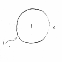
We started with two sets, but here let’s start with one. We’ll represent it as a circle on the plane. Call this circle c1.
Everything is either in the circle or outside it. It divides the plane into two regions. We’ll label the region inside the circle 1 and the region outside (the rest of the plane) x.
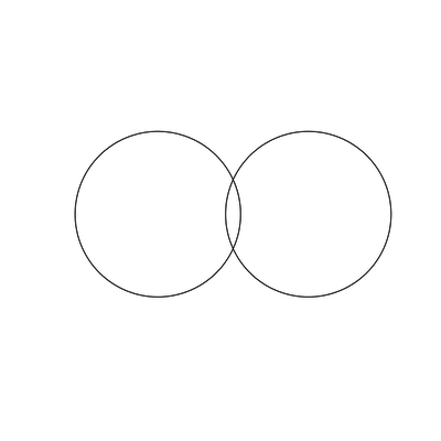
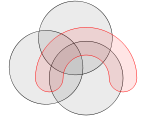
Now let’s look at two sets, which is probably the default Venn diagram everyone thinks of. Here we have two intersecting circles, c1 and c2.
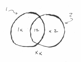
We need to consider both circles when labelling the regions now. For everything inside c1 but not inside c2, use 1x; for the intersection use 12; for what’s in c2 but not c1 use x2; and for what’s outside both circles use xx.
We can put this in a table:
| 1 | 2 |
|---|---|
| 1 | x |
| 1 | 2 |
| x | 2 |
| x | x |
This looks like part of a truth table, which of course is what it is. We can use true and false instead of the numbers:
| 1 | 2 |
|---|---|
| T | F |
| T | T |
| F | T |
| F | F |
It takes less space to just list it like this, though: 1x, 12, x2, xx.
It’s redundant to use the numbers, but it’s clearer, and in the elementary school math class they were using them, so I’ll keep with that.
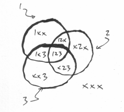
Three circles gives eight regions: 1xx, 12x, 1x3, 123, x2x, xx3, x23, xxx.
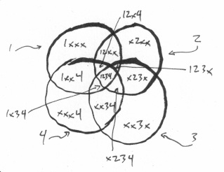
Four intersecting circles gets busier and gives 14 regions: 1xxx, 12xx, 123x, 12x4, 1234, 1xx4, 1x34, x2xx, x23x, x324, xx3x, xx34, xxx4, xxxx.
Here N and I stopped and made a list of circles and regions:
| Circles | Regions |
|---|---|
| 1 | 2 |
| 2 | 4 |
| 3 | 8 |
| 4 | 14 |
When N saw this he wondered how much it was growing by each time, because he wanted to know the pattern. He does a lot of that in school. We subtracted each row from the previous to find how much it grew:
| Circles | Regions | Difference |
|---|---|---|
| 1 | 2 | |
| 2 | 4 | 2 |
| 3 | 8 | 4 |
| 4 | 14 | 6 |
Aha, that’s looking interesting. What’s the difference of the differences?
| Circles | Regions | Difference | DiffDiff |
|---|---|---|---|
| 1 | 2 | ||
| 2 | 4 | 2 | |
| 3 | 8 | 4 | 2 |
| 4 | 14 | 6 | 2 |
Nine-year-old (almost ten-year-old) N saw this was important. I forget how he put it, but he knew that if the second-level difference is constant then that’s the key to the pattern.
I don’t know what triggered the memory, but I was pretty sure it had something to do with squares. There must be a proper way to deduce the formula from the numbers above, but all I could do was fool around a little bit. We’re adding a new 2 each time, so what if we take it away and see what that gives us? Let’s take the number of circles as n and the result as ?(n) for some unknown function ?.
| n | ?(n) |
|---|---|
| 1 | 0 |
| 2 | 2 |
| 3 | 6 |
| 4 | 12 |
I think I saw that 3 x 2 = 6 and 4 x 3 = 12, so n x (n-1) seems to be the pattern, and indeed 2 x 1 = 2 and 1 * 0 = 0, so there we have it.
Adding the 2 back we have:
Given n intersecting circles, the number of regions formed = n x (n - 1) + 2
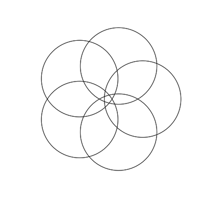
Therefore we can predict that for 5 circles there will be 5 x 4 + 2 = 22 regions.
I think that here I drew five intersecting circles and counted up the regions and almost got 22, but there were some squidgy bits where the lines were too close together so we couldn’t quite see them all, but it seemed like we’d solved the problem for now. We were pretty chuffed.
When I got home I got to wondering about it more and wrote a bit of R.
I made three functions; the third uses the first two:
circle(x,y): draw a circle at (x,y), default radius 1.1roots(n): return the n nth roots of unity (when using complex numbers, x^n = 1 has n solutions)drawcircles(n): draw circles of radius 1.1 around each of those n roots
circle <- function(x, y, rad = 1.1, vertices = 500, ...) {
  rads <- seq(0, 2*pi, length.out = vertices)
  xcoords <- cos(rads) * rad + x
  ycoords <- sin(rads) * rad + y
  polygon(xcoords, ycoords, ...)
}

roots <- function(n) {
  lapply(
    seq(0, n - 1, 1),
    function(x)
      c(round(cos(2*x*pi/n), 4), round(sin(2*x*pi/n), 4))
  )
}

drawcircles <- function(n) {
  centres <- roots(n)
  plot(-2:2, type="n", xlim = c(-2,2), ylim = c(-2,2), asp = 1, xlab = "", ylab = "", axes = FALSE)
  lapply(centres, function (c) circle(c[[1]], c[[2]]))
}
drawcircles(2) does what I did by hand above (without the annotations):
drawcircles(5) shows clearly what I drew badly by hand:
Pushing on, 12 intersecting circles:
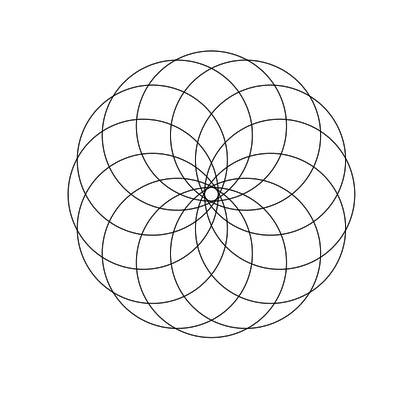
There are 12 x 11 + 2 = 123 regions there.
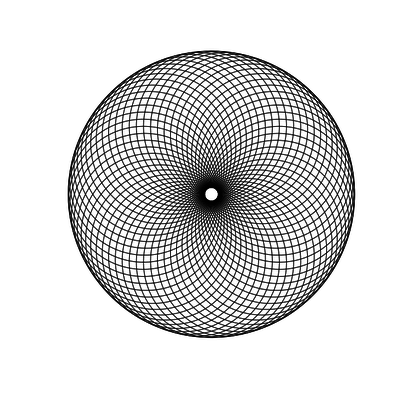
And 60! This has 60 x 59 + 2 = 3598 regions, though at this resolution most can’t be seen. Now we’re getting a bit op art.
This is covered in Wolfram MathWorld as Plane Division by Circles, and (2, 4, 8, 14, 24, …) is A014206 in the On-Line Encyclopedia of Integer Sequences: “Draw n+1 circles in the plane; sequence gives maximal number of regions into which the plane is divided.”
Somewhere along the way while looking into all this I realized I’d missed something right in front of my eyes: the intersecting circles stopped being Venn diagrams after 3!
A Venn diagram represents “all possible logical relations between a finite collection of different sets” (says Venn diagram on Wikipedia today). With n sets there are 2^n possible relations. Three intersecting circles divide the plane into 3 x (3 - 1) + 2 = 8 = 2^3 regions, but with four circles we have 14 regions, not 16! 1x3x and x2x4 are missing: there is nowhere where only c1 and c3 or c2 and c4 intersect without the other two. With five intersecting circles we have 22 regions, but logically there are 2^5 = 32 possible combinations. (What’s an easy way to calculate which are missing?)
It turns out there are various ways to draw four- (or more) set Venn diagrams on Wikipedia, like this two-dimensional oddity (which I can’t imagine librarians ever using when teaching search strategies):
You never know where a bit of conversation about Venn diagrams is going to lead!